This website uses cookies to ensure you get the best experience on our website.
- Table of Contents
This page contains information on how to perform ELISA data. If you are looking for a tool online to analyze ELISA data in an one-click fashion, please check out our newest tool for ELISA data analysis below.
Take me to ELISA data analysis toolELISA is a plate-based assay used to detect the concentration of a target protein in biological samples such as peptides, proteins, antibodies and hormones. Three different types of data output can be acquired:
Qualitative: Simply obtain a yes or no answer to the presence of the target protein in the sample by comparing to the blank well or an unrelated control antigen without the target protein
Semi-Quantitative: Use the signal intensities to compare the relative levels of the target protein in the assay samples since signal intensity is directly related to antigen concentration
Quantitative: Precisely calculate the target protein concentration in assay samples by comparing to a standard curve with known target protein concentrations that have been serially diluted
After performing an ELISA with a ready-to-use ELISA kit or an antibody pair kit, the data generated must be analyzed to quantitate the target protein concentrations.
Below, we discuss the different aspects to consider for more consistent and accurate ELISA data. Furthermore, we provide a step-by-step guide to create the standard curve for analysis.
Get a unique combination of service quality and subject expertise by outsourcing your ELISA experiments to Boster Bio.
Before running an ELISA, we recommend performing some best practices:
A standard curve (aka calibration curve) for the protein of interest is constructed by plotting the mean absorbance (y-axis) against the protein concentration (x-axis) and choosing the best fit curve for the data points. Based on the standard curve, we interpolate the sample absorbances to compute the sample concentrations. We will be discussing the steps in more detail below.
After obtaining raw data from the ELISA reader, the ELISA results are ready for statistical analysis. We suggest using an ELISA data analysis software for the analysis. Our lab works with CurveExpert 1.4, but many other curve fitting software and tools are available, such as GraphPad Prism. Microsoft Excel can also be used to analyze ELISA results, but it may not offer as many options or flexibility as other programs for scientists.
For this standard curve example, we will be using CurveExpert 1.4 to explain the process.
Categorize the ELISA raw data into three sections:
It is important to run the blank well with sample diluent to determine the background absorbance. Even without the presence of the protein, the buffer will still have an OD value. The absorbance of the blank wells should be subtracted from all standard and sample absorbances for accurate OD readings.

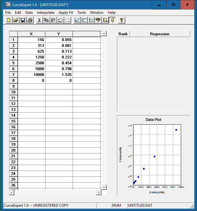
As an example, using Human DEFA1 PicoKine™ ELISA Kit (Catalog # EK1514), the mean absorbance of the blank well has been subtracted for all standards and samples
Open “CurveExpert 1.4” to see the interface below:
Enter the standard concentration in the x-axis column and the corresponding OD values in the y-axis column. The data plot will be presented in the bottom right corner.
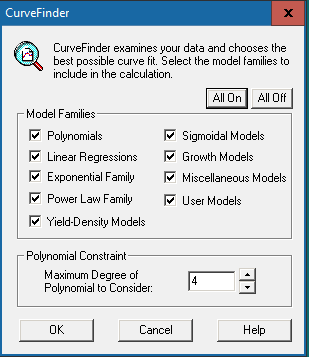
Click the [Run] button  in the top menu bar to allow the software to examine the data and choose the best possible curve fit. The window below will show up:
Click [All On] to include all model families for calculation. However, if you prefer not to include all of them, specific model families can also be selected for calculation. If “Polynomials” is checked, you will be asked to input the polynomial constraint, which we recommend setting as “4”.
Press [OK] to run the calculation.
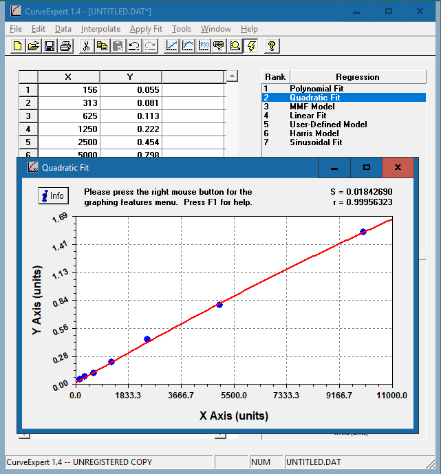
The resulting curve fits will be ranked based on the standard error and correlation coefficient. Double click on each model to see the corresponding curve.
Choose the curve that meets the following criteria:
Right click and select “Copy” to paste the graph into an excel sheet or word document.
Our lab and most companies generally recommend using a 4-parameter algorithm for the best standard curve fit. [Why?]
In this example, we have chosen the quadratic fit curve. Apart from the polynomial fit, the quadratic curve has the highest R value and closely resembles a straight line that rises smoothly. [Why aren’t we using the polynomial fit curve?]
The calculation can be performed in the software or with Excel. If the samples were diluted before the ELISA, make sure to multiply the computed sample concentrations by the sample dilution factor.
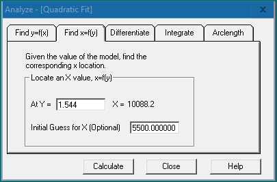
Using software will enable the user to easily find the x- and y-values, differentiate, and integrate the curve fit. Right click on the chosen curve fit graph for the graphing features menu and choose “Analyze”. For ELISA analysis, we would navigate to the “Find x=f(y)” tab and enter the sample OD value (y value) in the “At Y =” field. Click [Calculate] to obtain the x value (the target protein concentration) at the specified y value.
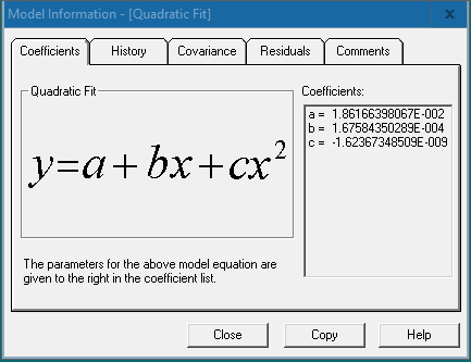
Click the [Info] button  in the top left corner of the graph. This will provide the model information for the curve fit along with other statistical information for the model.

The “Coefficients” tab displays the model function and the values of the coefficients a, b, c, etc. Press [Copy] and paste the function and coefficient values in an Excel sheet.
In the Excel sheet, input the corresponding coefficient values and y values (OD value) into the formula to calculate the sample concentrations.
Feel free to contact us if you encounter issues with your ELISA data analysis. We will be happy to assist you!
Curve fitting software will provide different model options for data plotting, including linear plots, semi-log plots, log/log plots, and 4- or 5-parameter logistic (4PL or 5PL) curves. Although linear plots with R2 values greater than 0.99 indicate good fitting, data points on the lower end of the range are compressed, which will reduce resolution. Semi-log and log/log plots resolve this issue. Data points are spread out more evenly with semi-log plots and log/log plots offer good linearity for the low to medium ranges of the curves. The 4- or 5-parameter logistic curves (4PL or 5PL) are more complex calculations that take into consideration additional parameters such as the maximum and minimum. The main difference between the 4PL and 5PL curves is that the 4PL curve is symmetrical around an inflection point, but the 5PL curve is asymmetrical. If the data points suggest asymmetry near the plateaus, the 5PL curve would be useful. However, more data points need to be collected to determine if asymmetry exists. As a result, it is generally recommended to use the simpler 4-PL for the best standard curve fit.
Although the polynomial fit curve is ranked 1 in the list and the curve has the highest R value for the example above, we should avoid using the polynomial fit as the standard curve. One thing to keep in mind with polynomials is that data points may sometimes result in a fitted curve that reaches maximum OD and then goes down again. This will result in having two concentration values for the same OD value. For example, the 2 polynomial curves shown below are unsuitable to be used as the standard curves for your ELISAs.


Learn the concept behind ELISA assay. Get to know how to maximize the sensitivity and precision of the assay, the plate must be carefully coated with high-affinity antibodies – a process that Boster Bio has mastered.

ELISAs can accurately assess soluble proteins in their native state, so they are ideal for samples such as urine or saliva. Check out the ELISA sample preparation guides to learn how to get the best results from your sample type.

Learn a stepwise ELISA protocol from reagent preparation to data analysis. Check out our ELISA protocols to learn how to get the best results.
![]()
Learn how to perform ELISA data analysis. Get to know the different aspects to consider for more consistent and accurate ELISA data. Furthermore, we provide a step-by-step guide to create a standard curve for analysis

