How to Quantify a Western Blot

Western blot “quantification” is often treated like a software task. In reality, most wrong numbers come from two upstream issues: saturation (signal no longer scales with protein amount) and normalization (a reference that shifts or saturates). The goal is not “the darkest band,” but measurable signal in the linear range with a defensible reference—so your fold change reflects biology, not imaging artifacts.

This post is a practical, 5-minute workflow for western blot quantification: capture a quantifiable image, measure band intensity (densitometry), normalize (loading control or total protein), and calculate fold change. If you want broader context or need to fix blot quality first, these internal hubs are designed to be your next clicks:

• Western blotting technical resource center
• Western blot troubleshooting library
• Total protein normalization vs loading control antibodies (TPS vs LC)

Quick answer: how to quantify a Western blot

Start with 3 questions: linear range, reference, and baseline

Most quantification confusion disappears when you answer three questions up front: Are my signals in the linear range? What will I normalize against? What am I calling “1×”? The best workflow is the one that keeps the blot measurable, uses a reference that doesn’t mislead, and defines fold change clearly.

1) Are my bands in the linear range (no saturation)?

If a target band (or your reference band) is saturated, intensity stops scaling with protein amount. Densitometry will still produce a number, but it won’t represent biology. A practical habit is to capture 2–3 exposures (or equivalent settings) and quantify the image where bands are clear without clipping.

2) Will I normalize to a loading control or total protein (TPS)?

Loading controls can work, but they can also saturate easily and sometimes change with treatment. Total protein normalization (TPS) often has a wider linear range and can be more robust in complex biology. If you want the deeper rationale, see TPS vs loading control antibodies.

3) What is my baseline for fold change?

Fold change only makes sense when your baseline is explicit. The most common baseline is the mean of the control group in the same experiment (same blot set, same imaging rules).

Quick takeaway

Step 1: capture an image you can actually quantify

Checklist: before you quantify (2-minute setup)

Same blot, different exposures (linear range vs saturation)

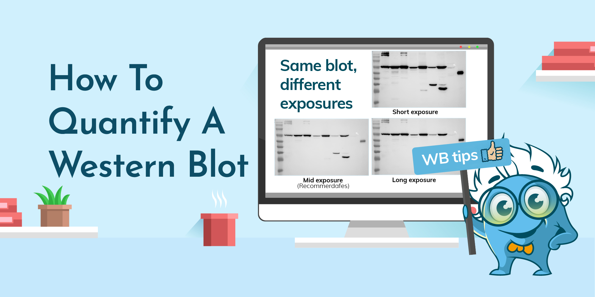
Short exposure (underexposed)

Mid exposure (recommended for quantification)

Long exposure (risk of saturation)

Same blot, different exposures. Darker bands at long exposure do not always mean “more protein.” Once signal approaches saturation, intensity stops scaling with protein amount. For quantification, choose the clearest non-saturated exposure and keep the same imaging settings across samples. (Click any image to open full-size.)

Same blot, different exposures. Darker bands at long exposure do not always mean “more protein.” Once signal approaches saturation, intensity stops scaling with protein amount. For quantification, choose the clearest non-saturated exposure and keep the same imaging settings across samples.

Quantification failures typically start at imaging. Capture a short exposure series and choose the image where bands are visible but not clipped. Keep settings identical across the samples you compare. Save a lossless file. These habits protect your measurement before any software step.

Step 2: measure band intensity (densitometry) in ImageJ the consistent way

You don’t need to be an ImageJ power user for reliable densitometry. The workflow is simple: keep preprocessing minimal, measure bands with consistent ROIs, subtract background consistently, then export values for transparent calculations.

Start with minimal preprocessing. Convert to grayscale if needed. If your imaging produces bright bands on a dark background, you may invert so bands appear as peaks; this is optional. Avoid filters, sharpening, or lane-by-lane edits.

Now define your region of interest (ROI) in a way you can defend. Draw a rectangle that fully covers the target band in the first lane, then reuse that same ROI size for the same band across all lanes. Do not resize the rectangle to “fit” each band—ROI consistency is the point.

For background subtraction, place a same-sized background ROI in the same lane, close to the band, in a clean area with no signal. Subtract that value from the band ROI to obtain a background-corrected intensity. Then use gel analysis tools (lane profiling / peak area or integrated density) to read band intensity and export the numbers to a spreadsheet.

If your blot shows heavy smears, multiple ambiguous bands, or obvious non-specific signal, it’s usually faster to optimize specificity and background first (see the WB troubleshooting library) than to defend a precise measurement of the wrong band.

Step 3: normalize (LC vs TPS) — two options, one decision rule

Normalization makes lanes comparable. In most cases, you only need two paths: loading control normalization or total protein normalization (TPS). The correct choice depends on stability and signal range.

Option A: Loading control normalization. Divide target intensity by a housekeeping band in the same lane. This is valid when the housekeeping protein is stable under your conditions and its signal is not saturated.

Option B: Total protein normalization (TPS). Normalize to total lane protein. TPS is especially useful when housekeeping proteins may vary with treatment, when loading controls are too abundant and prone to saturation, or when biology broadly changes cellular state.

Quick decision Choose LC vs TPS in 60 seconds

Step 4: calculate fold change (transparent, copy-ready formulas)

Worked example: if your treated sample has corrected target = 18,500 and corrected reference = 9,250, the normalized value is 2.00. If your control group’s normalized mean is 1.00, the treated fold change is 2.0×. The most convincing upgrade isn’t a fancier analysis—it’s biological replication and a clearly defined baseline.

Troubleshoot quantification fast: failure signals and quick fixes

FAQ (common search questions)

How do you quantify a western blot?

Use densitometry on a non-saturated image to measure band intensity, subtract a consistent local background, normalize to a stable reference (loading control or TPS), then compute fold change relative to the control mean.

What is the linear range, and how do I avoid saturation?

The linear range is where intensity scales with protein amount. Avoid saturation by capturing multiple exposures and quantifying the image where bands are clear without clipping. Make sure your reference (LC or TPS) is also non-saturated.

Should I normalize to housekeeping or total protein (TPS)?

Use a loading control if it’s stable under your condition and not saturated. Use TPS if housekeeping may change with treatment or saturates easily, or when biology broadly changes cellular state. See the TPS vs LC deep-dive for details.

How should I choose background for densitometry?

Use a same-sized ROI in the same lane, close to the band, in a clean area with no signal. Apply the same rule across all lanes and samples.

Checklist: 10-second final QC before you publish