This website uses cookies to ensure you get the best experience on our website.


- Table of Contents
You start adding reagent to a 96-well plate, move steadily across the rows or columns, and reach the last well more than ten minutes after the first. The immediate concern is obvious: has the first part of the plate already reacted long enough to bias the result?
Sometimes yes, but the elapsed time between the first and last addition is not the quantity that matters most. What matters is the reaction time experienced by each well: when that step began, and when it actually ended.
If a step is started and ended in the same order and at roughly the same pace, much of the offset cancels. If the ending sequence does not match the starting sequence, the first wells may receive a longer effective incubation or development window than the last wells. That difference is especially important during enzyme-substrate development, where signal is still accumulating minute by minute.
Core point: The practical problem behind ELISA pipetting order timing drift is not that every well starts at the same clock time, but whether the plate is handled in a way that gives some wells systematically more reaction time than others.
Consider the substrate step. Suppose TMB reaches the first well at minute 0 and the last well at minute 10. If stop solution is then added in the same sequence, beginning with the first well and ending with the last, each well can still receive about the same development interval. The clock times differ, but the reaction windows are similar.
The problem appears when the plate is ended on a different schedule. If every well is stopped at minute 20 from the first addition, the first well has developed for 20 minutes while the last has developed for only 10. The plate now contains a built-in timing gradient before any biological difference is considered.
Reviewing the full sandwich ELISA workflow can help identify exactly which event starts and ends each incubation.
The same ten-minute difference does not carry the same risk at every stage of an ELISA. Long binding incubations are often relatively forgiving; active color development is not.
| ELISA step | Typical sensitivity to timing differences | Why it matters |
|---|---|---|
| Sample incubation | Low to moderate | Long incubations often approach a binding plateau. |
| Detection antibody incubation | Low to moderate | A few extra minutes usually matter less once binding has slowed. |
| Enzyme conjugate incubation | Moderate | Unequal binding time can change the amount of active enzyme retained. |
| Substrate development | High | Color continues to accumulate while the enzyme-substrate reaction is running. |
| Stop solution addition | High | This defines when substrate development ends in each well. |
| Washing | Different kind of risk | Residual volume, soak time, aspiration consistency, and drying often matter more than elapsed time alone. |
Antigen capture, detection-antibody binding, and conjugate binding are association reactions. They are commonly given much longer incubation periods than the time required to pipette across one plate. As those reactions move toward a plateau, an extra few minutes usually changes the signal less than the same extra time during active color development.
That does not make long incubations immune to timing effects. Incubation conditions can still change measured concentrations, as shown in work such as Thuroczy et al. (2016). It simply means that a ten-minute delay during a long antibody incubation should not be treated as equivalent to a ten-minute difference in TMB development.
If you are pipetting TMB manually with a multichannel pipette, this is the point in the assay where plate order becomes easiest to see in the final OD values. The enzyme in each well keeps converting substrate until stop solution arrives. A well that develops longer can therefore read higher even when it contains the same amount of analyte.
The effect is not necessarily linear across the whole signal range. Once high-signal wells approach the upper part of the reader range, additional development time may change absorbance differently from low- or mid-range wells. This is one reason the substrate window should be defined in advance and kept inside the assay working range rather than judged by eye. These considerations are part of routine ELISA optimization.
Practical rule: If substrate is added from Column 1 to Column 12, add stop solution from Column 1 to Column 12 at a similar pace. Reversing the order, pausing midway, or stopping the entire plate on one clock time can quickly create different development windows.
Random pipetting error tends to scatter. Timing drift tends to follow the route the pipette took. If the plate was filled from left to right, OD may gradually rise or fall from the early columns to the late ones. If the plate was filled down rows, the same pattern can appear vertically.
This is also why adjacent duplicates can look reassuring even when the plate has a larger positional problem. Two neighboring wells were handled only seconds apart, so their agreement may be excellent. Replicates separated across the fill path are more likely to reveal a gradual timing gradient.
The standard curve is where a positional difference can become more consequential. If calibrators occupy the early part of the plate and unknowns occupy the late part, unequal development windows can put the two regions on different signal scales. Because ligand-binding curves are nonlinear, the resulting concentration error is not necessarily a constant shift that can be fixed afterward. Findlay and Dillard (2007) discuss why calibration-curve fitting itself affects back-calculated accuracy; a timing gradient adds another source of distortion.
When a plate looks suspicious, look at the raw OD by well position before focusing only on the calculated concentration. The ELISA data analysis guide is useful for checking the standard curve, replicate agreement, and the conversion from absorbance to concentration.
Not every row or column pattern comes from timing. Evaporation, temperature equilibration, washing, and instrument position can all create structured variation across a 96-well plate. The useful clue is whether the pattern follows the pipetting sequence or stays attached to a physical part of the plate.
A timing effect should move when the fill direction moves. If you run a uniform sample from left to right on one plate and right to left on another, a genuine order-related gradient should reverse. An edge effect usually will not: the outer wells remain the outer wells regardless of which direction you pipette. Mansoury et al. (2021) and Gregory and Sun (2009) describe evaporation-related edge effects in microplate work.
Washing can create a different pattern again. Uneven aspiration, different soak times, residual liquid, or partial drying may produce strip-wise or irregular effects that do not cleanly track the reagent-addition path. If the pattern is not convincingly directional, compare it with the other failure modes in the ELISA troubleshooting guide before assigning the problem to timing.
You do not need an automated workstation to control plate timing, but the sequence should be decided before the timed step begins. Prepare the reagent, reservoir, timer, and stop solution first. Use a multichannel pipette or repeating dispenser when possible so the first-to-last interval is shorter and more reproducible.
More important than speed is consistency. Start and end a timed step in the same direction. Avoid a long interruption halfway through the plate. For substrate development, time the reaction deliberately rather than starting a timer only after every well has already received substrate.
Plate layout matters as well. Loading all controls first, all treated samples second, and all remaining groups last may be convenient, but it also makes experimental group follow pipetting order. If a timing gradient is present, the technical effect and the biological comparison become difficult to separate. Distributing groups across the plate, rather than blocking them strictly by fill order, reduces that risk.
For assays that will be repeated over time, record the fill direction, substrate-development sequence, QC performance, and any visible positional pattern as part of the assay documentation. A simple note on the plate map can make a recurring problem much easier to recognize later. Boster’s ELISA validation information provides additional context for documenting assay performance.
A plate does not need to be discarded simply because dispensing took several minutes. If the delay occurred during a long binding incubation, the step was ended in the same sequence in which it was started, standards and controls look normal, and there is no directional OD trend, the timing gap alone may not justify a repeat.
I would be more cautious when the delay occurred during substrate development, especially if substrate and stop solution were added in different orders. A progressive OD shift from the first columns to the last is another warning sign. The concern is higher still if standards and unknowns occupy different regions of that gradient, because the timing effect can then influence the calibration relationship as well as individual sample signals.
A reversed-order repeat is one of the cleanest checks. If the high and low ends swap when the fill direction is reversed, order is strongly implicated. If the same physical wells stay abnormal, look harder at evaporation, washing, temperature, or the instrument. Uniformity-style checks are useful here because any structure in a plate filled with the same material must be technical rather than biological; this general approach is consistent with plate-uniformity thinking used in assay validation (Zhang et al., 1999).
When several timing warning signs occur together, repeating the plate under controlled conditions is usually easier to defend than trying to correct a gradient mathematically after the fact. Andreasson et al. (2015) and Lee et al. (2006) both emphasize that precision, recovery, and fitness for purpose depend on characterizing an assay under the conditions in which it is actually run.
The first and last well on a manually handled 96-well plate will rarely be treated at exactly the same moment. That alone is not the problem. The important question is whether those different start times turn into different reaction times.
Long binding steps often tolerate a modest plate-wide offset reasonably well, particularly when the step is ended in the same order in which it began. Substrate development deserves much closer control because signal continues to accumulate until stop solution is added. A mismatch between substrate order and stop order can therefore create a systematic gradient that looks like a real sample difference.
When investigating ELISA pipetting order timing drift, check three things: where the delay occurred, whether start and stop order matched, and whether the OD pattern follows the fill path.
Those three observations usually tell you more than the first-to-last clock difference by itself.
Good timing control is easier to interpret when the assay itself is standardized. Starting with validated PicoKine® ELISA kits provides characterized standards and reagents so that plate-handling effects can be evaluated against a consistent assay background.