How to Analyze ELISA Data and Calculate Results: Step-by-Step Guide with Troubleshooting Tips

I. Introduction

The Enzyme-Linked Immunosorbent Assay (ELISA) is a cornerstone technique in immunology and diagnostics, known for its sensitivity, specificity, and ability to detect a wide range of biomolecules. Despite its widespread use and standardized workflow, calculating and interpreting ELISA results can be complex, varying by assay type, kit manufacturer, and research purpose—each of which may follow slightly different procedural frameworks as seen in practical ELISA Testing Service implementations.

This guide provides a clear, practical overview of ELISA data analysis, from choosing the right curve-fitting model to determining when qualitative, semi-quantitative, or full quantitative interpretation is appropriate. It also includes ELISA troubleshooting tips to help ensure reliable and reproducible results. Whether you're new to ELISA or looking to improve your assay accuracy, this article will support your efforts with proven strategies and tools.

Before diving into calculation details, it can also be helpful to review an ELISA experimental design checklist so assay format, controls, standards, dilution planning, and plate reading decisions are aligned before the run begins.


II. Why ELISA Calculation Methods Differ


1. Differences in ELISA Types

Although the core principle of ELISA is the detection of a specific molecular interaction—typically between an antigen and an antibody—there are multiple assay formats, each with distinct detection mechanisms. These differences directly influence how results should be calculated and interpreted.

The most common ELISA types include:

  • Sandwich ELISA – Typically used for quantifying proteins or cytokines. The signal (OD value) increases proportionally with the concentration of the target analyte.
  • Competitive ELISA – Often used for small molecules or hormones. The signal (OD value) decreases inversely as analyte concentration increases.
  • Indirect ELISA – Common for antibody detection. Signal increases with antibody presence, but may be less linear than sandwich ELISA.
  • Direct ELISA – A simplified version of indirect ELISA, mostly used for qualitative or semi-quantitative purposes.
  • Multiplex ELISA kits – Allow simultaneous detection of multiple targets in a single sample. While the data output is more complex, the calculation principle for each individual target remains similar to single-target ELISA (e.g., using standard curves per analyte). However, analysis often requires specialized software due to multiple detection channels.

If you are still deciding which assay structure best fits your analyte, sensitivity target, and downstream readout, this guide on which ELISA is for you is a useful companion before locking in the analysis strategy.

Understanding your ELISA format is the first step in choosing the right data analysis strategy.


2. Relationship Between OD and Analyte Concentration

At the core of ELISA result interpretation lies the relationship between optical density (OD) and target concentration. This relationship varies depending on the ELISA format:

  • In sandwich, indirect, and direct ELISAs, OD values are positively correlated with analyte concentration. This is because the more target is present, the more enzyme-linked detection antibody can bind, producing a stronger colorimetric signal.
  • In competitive ELISA, OD values are negatively correlated. In this format, the target analyte in the sample competes with a labeled version for limited binding sites. A higher concentration of sample analyte results in less binding of the labeled antigen, producing a weaker signal.

3. Differences in Curve-Fitting Models and Analysis Tools

ELISA kits from different manufacturers may recommend different methods for fitting the standard curve, depending on the assay range and expected sensitivity:

  • Linear regression is sometimes used for narrow ranges with near-linear OD–concentration relationships.
  • Logarithmic (log–log) plots are common in kits with exponential response curves.
  • 4-parameter logistic (4PL) and 5-parameter logistic (5PL) models are the most widely used and accurate for fitting ELISA standard curves across a wide dynamic range.

For a more detailed walkthrough of standard preparation, concentration gradients, and graph construction, see how to generate an ELISA standard curve.

While researchers can manually fit curves using tools like Microsoft Excel or GraphPad Prism, there are also excellent online platforms that simplify the process:

III. Qualitative and Semi-Quantitative Analysis Methods


1. When to Use Qualitative Analysis

Qualitative interpretation (positive vs negative) is suitable when the goal is to detect the presence or absence of a target, rather than its exact concentration. Typical scenarios include:

  • Disease diagnostics – e.g., presence of viral antigens or antibodies
  • Antibody screening – such as hybridoma supernatant selection
  • Protein expression verification – confirming whether a transgene or antigen is present

2. How to Set a Cutoff Value

To determine whether a sample is positive or negative, a cutoff OD value must be established. Common methods include:

  • Statistical approach:
    Cutoff = Mean OD of negative controls + 2 × Standard Deviation (SD)
  • Kit-specific threshold:
    Some commercial ELISA kits provide manufacturer-defined cutoff values based on validation studies.

If you need a more practical breakdown of what each control is actually telling you, including process blank, true negative, and spike-based checks, this guide on ELISA controls that actually matter can help tighten interpretation.

Interpretation:

  • OD > Cutoff → Positive
  • OD ≤ Cutoff → Negative

This method offers a simple yet effective way to evaluate results in screening or diagnostic assays.


3. Semi-Quantitative Classification

In some studies, particularly when monitoring immune responses or comparing relative expression, semi-quantitative grading is helpful. Rather than reporting precise concentrations, samples are categorized by signal strength:

  • Weak positive: OD slightly above the cutoff
  • Moderate positive: OD about 2–3× the cutoff
  • Strong positive: OD > 3× the cutoff

This approach is commonly used in:

  • Antibody titer assessment
  • Vaccine response monitoring
  • Preliminary high-throughput ELISA screens

IV. Standard Quantitative Analysis Workflow

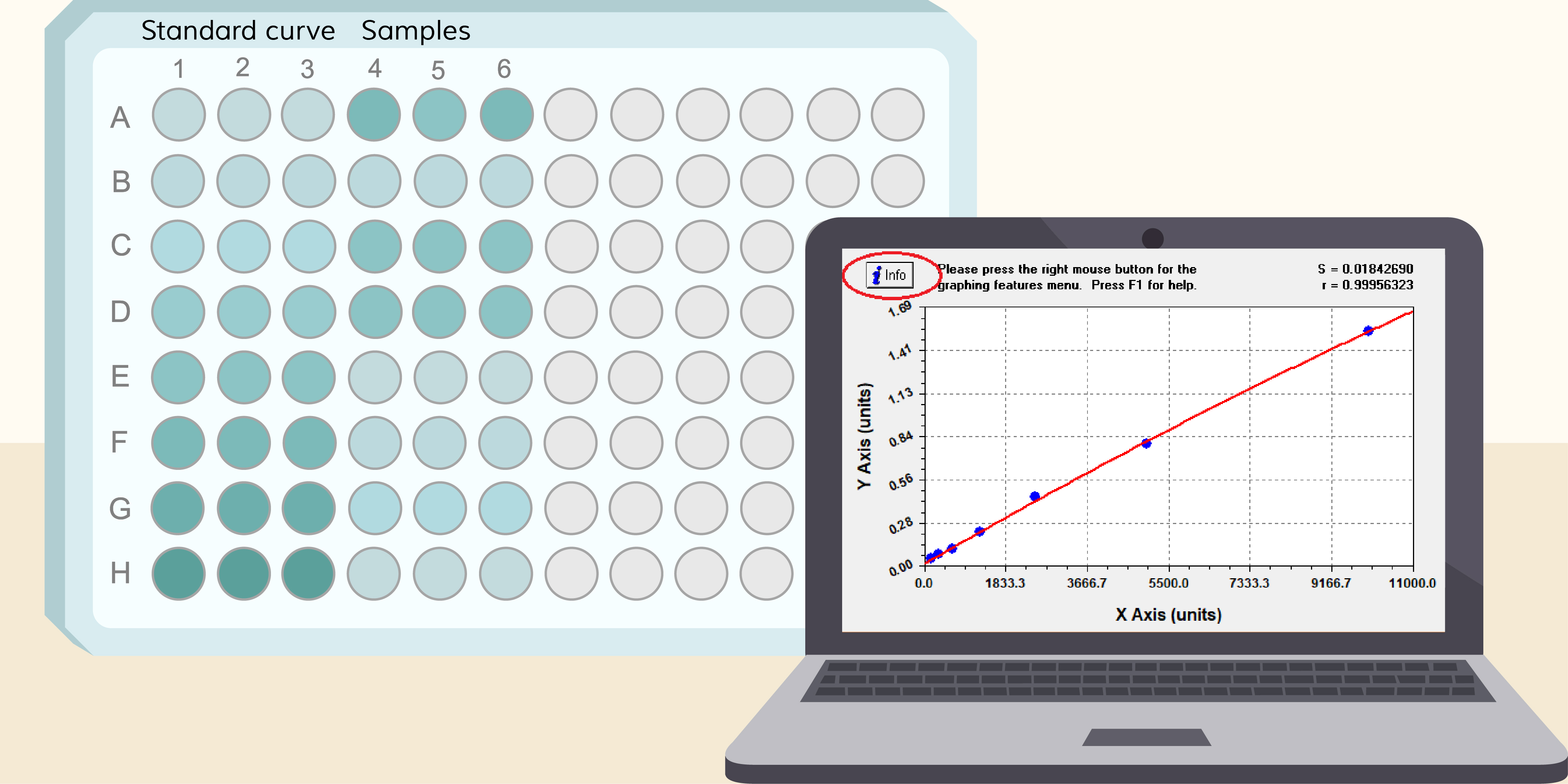
Quantitative ELISA allows researchers to determine the absolute concentration of a target analyte in unknown samples by comparing their optical density (OD) values to a standard curve generated from known concentrations. This section provides a step-by-step guide to ensure accurate and reproducible quantification.


1. Preparing Standards and Plotting the Standard Curve

a. Serial Dilution Strategy
  • Prepare a series of 2-fold, 3-fold, or 5-fold dilutions from a high-concentration standard.
  • For most ELISA kits, the highest standard is typically between 1000–5000 pg/mL, depending on the target.
  • Use assay buffer (or the same matrix as your sample) to dilute.

If you want a dedicated walkthrough for concentration gradients, blank setup, and standard-point arrangement, refer to how to generate an ELISA standard curve.

b. Recommended Concentration Range
  • Ensure the range covers the expected sample values.
  • Include at least 6–8 standard points, plus a zero standard (blank).
  • If your samples come from blood-derived matrices, confirm early whether serum or plasma is more appropriate for the assay, since matrix-related interference can shift expected values and affect interpretation. This practical guide on serum or plasma for ELISA can help you troubleshoot that choice before it becomes a data-analysis problem.
c. Replicates
  • Run each standard in duplicate or triplicate to ensure consistency and identify pipetting errors.

2. Reading OD Values and Processing Raw Data

a. Plate Reading
  • Most ELISAs are read at 450 nm using a microplate spectrophotometer.
  • Some kits may include a reference wavelength (e.g., 570 or 630 nm) to correct for plate imperfections—if so, subtract the reference from the primary OD.
b. Background Subtraction
  • Subtract the OD of the blank well (zero standard) from all other readings to eliminate the background signal.
  • Adjusted OD = Sample OD – Blank OD

3. Curve Fitting Methods

Accurate fitting of the standard curve is essential for precise interpolation of sample concentrations.

a. Recommended Software
b. Curve Models
  • 4-Parameter Logistic (4PL): Best for most ELISAs due to its flexibility and sigmoidal fit.

Equation form:

The 4-parameter logistic (4PL) equation is:

Y = D + (A - D) / (1 + (X / C)B)

where A = minimum, D = maximum, C = inflection point (EC50), B = slope

  • 5PL: Adds asymmetry for curves with skewed distributions
  • Linear/logarithmic: Only acceptable if the OD–concentration range is narrow and the plot is linear.

4. Calculating Sample Concentrations

Once the standard curve is fitted:

a. Interpolation
  • Use the curve to interpolate the concentrations of unknown samples from their adjusted OD values.
  • Ensure that sample ODs fall within the range of the standard curve. If not, dilute the sample further.
b. Dilution Factor Correction
  • If samples were diluted during preparation, multiply the interpolated value by the dilution factor to recover the original concentration.
  • Final concentration = Interpolated value × Dilution factor

For a more practical workflow on choosing starting dilution, running a pilot serial dilution, and avoiding saturation or out-of-range readings, see how to decide ELISA dilution ratio.

c. Confirm Result Units
  • Most ELISA kits report results in pg/mL, ng/mL, or μg/mL.
  • Always check the standard concentration units and maintain consistency across calculations and reporting.

5. Quality Control Recommendations

Ensuring accuracy and reproducibility is critical in quantitative ELISA analysis.

a. Coefficient of Variation (CV%)
  • Intra-assay CV% (within the same plate) should be <10%.
  • Calculate CV% for replicates:
    CV% = (Standard Deviation ÷ Mean) × 100
b. Identifying and Handling Outliers
  • Check for replicate wells with unusually high variation.
  • Use Grubbs' test or similar statistical tests to flag outliers if needed.
  • Repeat measurements for questionable wells if resources allow.
c. Curve Validation
  • The standard curve should have an R² > 0.99 when using appropriate models.
  • If the curve is poorly fitted, check for pipetting errors, contamination, or reagent instability.


When reproducibility problems persist despite a smooth curve, it is often useful to step back and review controls, dilution logic, and plate setup together using an ELISA experimental design checklist and a more focused control guide such as ELISA controls that actually matter.

V. Common Errors and Troubleshooting Tips

Even with well-validated ELISA kits and protocols, variability and errors can arise during the experiment. This section outlines frequent issues, explains their causes, and provides practical solutions.


1. Low OD Values or No Signal

Possible causes:

  • Missing key reagents (e.g., detection antibody, substrate)
  • Expired or degraded substrate (TMB)
  • Inadequate incubation (time or temperature)
  • Low antigen or antibody concentration
  • Over-washing that removes coated or captured molecules

Solutions:

  • Double-check pipetting sequence and reagent addition
  • Use fresh substrate
  • Validate incubation conditions
  • Optimize antibody/antigen concentrations

2. High Background or Non-Specific Signal

Possible causes:

  • Incomplete washing, leaving non-specific bindings
  • Excessive concentration of detection antibody
  • Inadequate blocking
  • Over-incubation or high incubation temperature

Solutions:

  • Increase wash cycles and ensure thorough aspiration
  • Dilute detection antibodies further
  • Use effective blockers (BSA, non-fat milk)
  • Shorten incubation time and optimize temperature

3. Poor Standard Curve Fitting

Possible causes:

  • Inaccurate standard dilutions
  • Inadequate range coverage or number of standard points
  • Poor OD distribution or nonlinear response

Solutions:

  • Calibrate pipettes and mix thoroughly
  • Include more points across a wide, expected concentration range
  • Use 4-parameter logistic (4PL) fitting for sigmoidal curves
  • Try trusted platforms like:
    GraphPad Prism
    Boster’s Online Tool

4. High Replicate Variation (High Intra-Assay CV%)

Possible causes:

  • Inaccurate pipetting, especially during critical additions
  • Cross-contamination when removing plate seal
  • Inhomogeneous sample (precipitation, layering)
  • Edge effects due to temperature or evaporation

Solutions:

  • Use multi-channel pipettes and consistent technique
  • Avoid touching the inner wall of wells
  • Mix samples before loading
  • Avoid using edge wells or fill them with buffer for insulation

5. Do I Need to Generate a New Standard Curve Every Time?

Answer: Yes, it is strongly recommended.

Even slight changes in lab conditions (e.g., pipetting technique, plate washing, ambient temperature) can affect the standard curve. Relying on a previous curve may result in significant errors in sample concentration calculations.

Problem Possible Cause Suggested Solution
OD too low or flat Missing reagents, substrate expired, low concentrations, under-incubation Check reagent setup, increase incubation, optimize concentrations
OD too high or background noisy Insufficient washing, too much detection Ab, over-incubation Wash more, dilute antibodies, optimize blocking/incubation
Bad standard curve fit Pipetting error, not enough points, non-sigmoidal range Use 4PL fitting, increase standards, check dilution accuracy
High CV% between replicates Pipetting inconsistency, sample inhomogeneity, cross-contamination Standardize pipetting, vortex samples, avoid edge wells, peel seals carefully
“Can I reuse old standard curve?” Environmental and technical variability No—always regenerate fresh standard curves per run
CV% still too high Scraping coating, poor sample quality, edge effects Avoid touching wells, pre-mix samples, use central wells only

VI.Conclusion

Accurate calculation of ELISA results is essential for obtaining reliable, reproducible data that can support meaningful biological conclusions. From understanding the type of ELISA used, to properly reading OD values and generating a high-quality standard curve, each step of the process requires careful attention. Determining whether your experiment calls for qualitative, semi-quantitative, or full quantitative analysis helps guide the appropriate interpretation strategy. Tools such as 4PL fitting and online ELISA analysis platforms—including Boster’s own analysis tool—can significantly streamline this workflow. Finally, being aware of common ELISA pitfalls and implementing best practices in pipetting, plate handling, and data analysis will minimize error and enhance your assay’s consistency. By following the methods outlined in this guide, researchers can improve the accuracy of their ELISA results and ensure greater confidence in their experimental findings.