How to Tell If Your ELISA Standard Curve Is Reliable Beyond R²

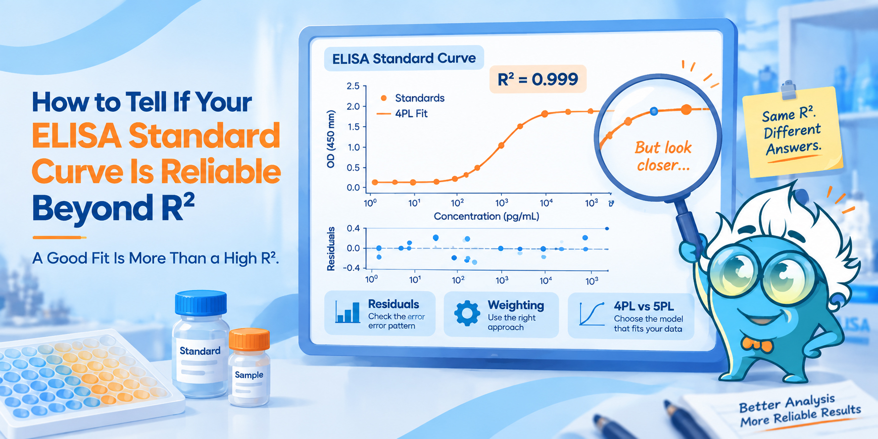
Most ELISA analysis software can generate a 4PL or 5PL standard curve in seconds. The curve may look smooth, the standards may appear close to the fitted line, and R² may be very close to 1.

That still does not tell you whether the fit is reliable enough for quantitation.

A reliable ELISA curve fit needs to do more than produce a smooth sigmoid and a high R². A curve can fit the data well overall while performing poorly in one part of the concentration range—and that matters if your samples fall in that region.

A more useful evaluation looks at residuals, back-calculated standards, and weighting. Residuals show where the model is missing the observed responses. Back-calculated standards show whether those misses translate into concentration error. Weighting becomes important when the variability of the response is not constant across the curve. [1–3]

For a broader workflow covering raw OD values, standard curves, and concentration calculations, see our guide to ELISA data analysis.

In This Article

1. Why ELISA Standard Curves Usually Need 4PL or 5PL Models
2. Why R² Is Not Enough for an ELISA Curve Fit
3. Residuals Show Where the Fit Is Missing the Data
4. Back-Calculated Standards Show Whether the Curve Is Quantitatively Reliable
5. Weighting Matters When Error Is Uneven Across the Curve
6. 4PL or 5PL? Let the Error Pattern Guide the Choice
7. Competitive ELISA Uses the Same Diagnostic Logic
8. A Practical Way to Review an ELISA Curve Fit
9. Residuals and Back-Calculation Together: A Curve-Fit Diagnostic Matrix
10. When the Problem Is Not Curve Fitting
11. What Should ELISA Curve-Fitting Software Let You Review?
12. How to Decide Whether an ELISA Curve Is Reliable
13. References
14. FAQs

1. Why ELISA Standard Curves Usually Need 4PL or 5PL Models

Across its full working range, a quantitative ligand-binding assay rarely produces a straight concentration-response relationship.

At the lower end, responses approach the lower asymptote. Through the middle of the curve, signal changes more rapidly with concentration. At the upper end, responses approach the upper asymptote. On a logarithmic concentration axis, this commonly produces the familiar sigmoidal relationship. [1,2]

The four-parameter logistic (4PL) model describes the two asymptotes, the inflection region, and the slope. One characteristic of the 4PL is symmetry around its inflection point. [2]

The five-parameter logistic (5PL) model adds an asymmetry parameter. This allows it to describe curves in which the two sides of the sigmoid are not symmetric, and can improve concentration estimates when genuine asymmetry is present. [2,5]

ICH M10 likewise notes that ligand-binding assay calibration curves are most often fitted with 4PL or 5PL models when data are available near both asymptotes. [4]

If you are still working on how to construct and fit the standards themselves, see how to generate an ELISA standard curve.

The presence of a fifth parameter, however, does not make 5PL automatically superior. If 4PL already describes the assay adequately, more flexibility may add little practical value. Published LBA recommendations favor a sufficiently simple model that provides adequate quantitative performance. [2,3]

2. Why R² Is Not Enough for an ELISA Curve Fit

R² is appealing because it reduces a complicated fit to one familiar number.

The limitation is that it does not tell you where the errors occur.

Two curves can have similar R² values while producing different errors in the concentrations calculated from them. Azadeh and colleagues specifically note that statistics such as R² evaluate fit in response space and do not necessarily reflect the quality of the reportable inverse prediction—the concentration you ultimately want to know. [2]

Suppose a curve has an R² of 0.999, but the lowest three standards are consistently displaced from the fitted curve.

If your unknowns sit near the middle of the range, the practical impact may be small. If most of your samples are close to the lower end, the same fitting behavior becomes much more important.

Residuals are one way to see where that question needs closer attention.

3. Residuals Show Where the Fit Is Missing the Data

A residual is the difference between the response observed for a standard and the response predicted by the fitted model:

If a standard produces an OD of 1.20 and the fitted model predicts 1.16, the residual is +0.04.

One residual is rarely informative by itself. The pattern across the curve is much more useful.

A well-behaved residual plot should not show persistent concentration-dependent bias. Published LBA recommendations describe random residual distribution without systematic bias at the low or high concentration levels as a desirable feature of model performance. [2]

What deserves attention is repeated structure.

If residuals tend to fall on one side of zero through one part of the range and shift to the other side elsewhere, the model may be missing something about the curve shape. Reproducible asymmetry is one possible explanation, although experimental problems should be considered before switching models.

A different pattern occurs when residual spread changes markedly across the response range. This is consistent with heteroscedasticity, or nonconstant response variance, which is well recognized in nonlinear ligand-binding calibration curves. [2,3] In that situation, weighting deserves closer examination.

An isolated large residual is different again. If one standard behaves poorly while adjacent concentrations do not, check the experimental point first. Replicate disagreement, a dilution error, pipetting, or another technical problem can make one standard look like a regression problem when it is not.

If standard preparation itself is questionable, the ELISA standard preparation guide is a better next step than immediately changing the regression model.

4. Back-Calculated Standards Show Whether the Curve Is Quantitatively Reliable

Residuals describe error in response units. ELISA results, however, are usually reported as concentrations.

Back-calculation connects the two.

Take a standard whose concentration is already known, treat its measured response as though it came from an unknown sample, and calculate its concentration from the fitted curve. You can then compare the result with the concentration that was actually prepared.

Findlay and Dillard recommend evaluating agreement between nominal and model-predicted calibrator values when assessing an LBA calibration model. [1] ICH M10 also requires reporting and evaluating back-calculated calibration-standard concentrations in regulated bioanalytical LBAs. [4]

Look Across the Curve, Not Only at One Failed Standard

These are diagnostic clues, not one-to-one diagnoses.

What Recovery Should an ELISA Standard Achieve?

There is no single acceptance threshold that should automatically be applied to every research-use ELISA.

For regulated ligand-binding bioanalytical assays, ICH M10 specifies that the accuracy and precision of back-calculated calibration-standard concentrations should be within ±20% of nominal at most levels and within ±25% at the LLOQ and ULOQ. At least 75% of calibration standards, excluding anchor points and including at least six concentration levels, should meet the specified criteria. [4]

Those thresholds belong to the regulated LBA context. They should not be presented as universal pass/fail rules for every exploratory or research-use ELISA.

For a research assay, the acceptance criteria should reflect the purpose of the experiment, assay performance, and predefined laboratory procedures.

5. Weighting Matters When Error Is Uneven Across the Curve

Nonlinear ligand-binding calibration curves frequently show unequal response variability across concentration levels. This is one reason an unweighted fit can perform well in one part of the curve while giving poorer inverse predictions elsewhere. [2,3]

Common options available in curve-fitting software include unweighted regression and weighting functions such as 1/Y and 1/Y².

The important point is not that one of these is universally preferable.

Weighting changes how different observations influence estimation of the curve parameters. The appropriate approach should be based on the assay’s response-error relationship and then assessed using quantitative performance, including the accuracy and precision of back-calculated concentrations. [2,3]

Xiang and colleagues presented three quantitative LBA case studies in which weighting functions were selected after evaluating heteroscedasticity, and the resulting weighted models were assessed using back-calculated %RE and %CV. The appropriate weighting differed among their assays. [3]

That is why 1/Y² should not be treated as a default answer to every poor ELISA curve.

If changing the weighting improves the low end but worsens concentration recovery elsewhere, the error has not necessarily been solved—it may simply have been redistributed.

After changing the weighting, go back to the same questions: Does the residual pattern improve? Do the standards back-calculate more appropriately? Does the fit perform better across the range that will actually be used?

6. 4PL or 5PL? Let the Error Pattern Guide the Choice

Most curve-fitting software makes it easy to switch between 4PL and 5PL. Selecting the model solely because one produces a slightly better R² is less useful.

A 4PL model is often sufficient when the calibration response is reasonably symmetric and quantitative performance across the intended range is acceptable.

A 5PL model becomes more relevant when the curve shows reproducible asymmetry. Gottschalk and Dunn showed that the additional asymmetry parameter can improve fitting and concentration estimation for asymmetric assay data. [5] Azadeh et al. similarly describe 5PL as an option when a symmetric 4PL does not adequately represent an asymmetric calibration curve. [2]

The important word is reproducible.

One unusual plate or one questionable standard is not strong evidence that the assay requires a five-parameter model.

If the 5PL improves the apparent fit but produces little meaningful improvement in back-calculated concentrations, the additional complexity may not be useful. Xiang et al. recommend comparing quantitative accuracy and precision between candidate models and favoring the simpler model when performance is comparable. [3]

7. Competitive ELISA Uses the Same Diagnostic Logic

In a noncompetitive assay such as a typical sandwich ELISA, the response is generally directly related to analyte concentration. In a competitive assay, the relationship can be inverse. [2]

The orientation of the sigmoid changes, but the diagnostic questions remain much the same.

You still need to know whether the model describes the standards appropriately, whether residuals show systematic bias, whether known concentrations can be recovered, and whether the weighting and quantitative range are suitable.

A descending calibration curve therefore does not require an entirely different philosophy of curve evaluation.

8. A Practical Way to Review an ELISA Curve Fit

A useful review can be reduced to five passes through the data.

1. Start With the Raw Standards

Before changing any fitting settings, look at replicate agreement, background, signal separation, saturation, and obvious dilution problems.

Many curve problems begin before the analysis stage. The ELISA experimental design checklist is useful when standards, controls, dilution strategy, or plate setup may be contributing.

2. Fit the Expected Model

If the assay already has an established analysis procedure, use it consistently. During assay development, begin with a justified model rather than trying multiple equations and choosing whichever produces the highest R². Both published best-practice recommendations and ICH M10 emphasize selecting an appropriate regression model during method development or validation. [2–4]

3. Review Residuals and Back-Calculated Standards Together

Residuals answer: Where is the model missing the observed response? Back-calculation asks: Does that error materially change the reported concentration? Neither needs to be treated as an isolated pass/fail metric.

4. Identify the Pattern Before Changing the Fit

If the problem is concentrated near one end of the range, investigate the assay signal, quantitative range, heteroscedasticity, and weighting. If residuals show reproducible shape-related bias, then a 4PL-versus-5PL comparison becomes more informative.

If samples themselves frequently fall outside the usable range, choosing an appropriate ELISA dilution may be more important than changing the regression equation.

5. Refit and Repeat the Same Checks

A model change should improve the problem that prompted the change without creating an unacceptable problem elsewhere. Do not stop simply because the new curve looks smoother.

9. Residuals and Back-Calculation Together: A Curve-Fit Diagnostic Matrix

Looking at residuals and back-calculated standards together is more informative than treating either one alone.

This matrix is intentionally diagnostic rather than prescriptive. The same visible pattern can have more than one cause, and the regression model should not be changed until the experimental data have also been reviewed.

10. When the Problem Is Not Curve Fitting

Curve-fitting software can draw a smooth line through imperfect data. That does not mean the assay itself behaved well.

If several high standards produce nearly indistinguishable responses, the problem may be saturation rather than regression. In that case, see the guide to ELISA saturated signals.

If the abnormality follows plate position—for example, perimeter wells behave differently from central wells—review ELISA edge effects before attributing the pattern to the curve model.

Standard preparation, poor replicate precision, washing or incubation variation, background, and other experimental problems can also distort calibration data. The ELISA troubleshooting guide provides a broader assay-level troubleshooting workflow.

Very high analyte concentrations can create another problem. ICH M10 specifically recommends evaluating dilution linearity and high-dose hook effect in ligand-binding assay validation because high concentrations can suppress signal and produce erroneous results. [4]

None of these problems can be fixed simply by adding another regression parameter.

11. What Should ELISA Curve-Fitting Software Let You Review?

A concentration table alone is not enough to evaluate a calibration model.

Ideally, the analysis environment should let you review the fitted curve alongside the observed standards and provide enough output to evaluate residual behavior, nominal versus back-calculated concentrations, quantitative accuracy, the selected regression model, and the weighting method being used. [2]

Not every ELISA analysis platform exposes all of these diagnostics. If your software only displays the fitted curve and R², additional statistical output may be needed before making decisions about model reliability.

For routine online ELISA data processing and concentration analysis, Boster provides an online ELISA data analysis tool. Use the diagnostic outputs available in your analysis software when evaluating residuals, weighting, and model performance.

12. How to Decide Whether an ELISA Curve Is Reliable

R² can remain part of your curve review. It simply should not make the decision by itself.

A stronger assessment combines three views of the same calibration curve:

• Residuals tell you where the fitted response departs from the observations.
• Back-calculated standards tell you how much that departure affects concentration estimates.
• Weighting and model choice tell you whether the error structure is being handled appropriately.

If the raw standards are sound, residual bias is limited, known concentrations are recovered adequately across the intended quantitative range, and alternative weighting or model choices do not reveal a meaningful improvement, the fit has much stronger support than a high R² alone can provide.

References

1. Findlay JWA, Dillard RF. Appropriate calibration curve fitting in ligand binding assays. The AAPS Journal. 2007;9(2):E260–E267. doi:10.1208/aapsj0902029.
2. Azadeh M, Gorovits B, Kamerud J, MacMannis S, Safavi A, Sailstad J, Sondag P. Calibration Curves in Quantitative Ligand Binding Assays: Recommendations and Best Practices for Preparation, Design, and Editing of Calibration Curves. The AAPS Journal. 2018;20:22. doi:10.1208/s12248-017-0159-4.
3. Xiang Y, Donley J, Seletskaia E, Shingare S, Kamerud J, Gorovits B. A Simple Approach to Determine a Curve Fitting Model with a Correct Weighting Function for Calibration Curves in Quantitative Ligand Binding Assays. The AAPS Journal. 2018;20:45. doi:10.1208/s12248-018-0208-7.
4. International Council for Harmonisation of Technical Requirements for Pharmaceuticals for Human Use. ICH M10: Bioanalytical Method Validation and Study Sample Analysis. Guidance for Industry. November 2022.
5. Gottschalk PG, Dunn JR. The five-parameter logistic: a characterization and comparison with the four-parameter logistic. Analytical Biochemistry. 2005;343(1):54–65. doi:10.1016/j.ab.2005.04.035.