Boster Bio Life Science Blog

How to Strip and Re-probe Cleanly

A verification-first workflow to prevent ghost bands and high background.

Western blot “failures” are often pinned on antibodies, transfer, or blocking. But when you’re stripping and re-probing, the make-or-break step is simpler: whether round one antibodies are truly removed without damaging what you’re trying to detect next. The goal is a verification-first stripping protocol that keeps signal-to-background high—so round two reads like biology, not carryover.

If you want broader context (or want to move downstream after your workflow is solid), these internal hubs are designed to be your next clicks:

• Full Western blot protocol
• Western blot troubleshooting library
• Western blot reagents
• Loading control antibodies
• Total protein normalization vs loading control antibodies
• Western blotting service

Stripping and re-probing is most useful when it replaces a full rerun—another gel, another transfer, and another antibody cycle—without compromising interpretability. The workflow below focuses on the two outcomes that matter most in practice: avoiding antibody carryover that becomes ghost bands, and preserving immobilized protein so your second-round signal doesn’t collapse into background.

When to use a western blot stripping buffer (and when to rerun instead)

Stripping is worth doing when reusing the membrane genuinely replaces a full gel/transfer cycle. But it can become a time sink when your first-round signal is already near the detection limit or your experiment requires strict quantitative comparability across conditions. When you’re unsure whether your problem is stripping-related or coming from upstream steps, it’s often faster to cross-check your baseline workflow against the Western blot troubleshooting library before you change stripping conditions.

Table 1. Strip & re-probe vs rerun: a decision guide

A practical rule that saves time: if the band is barely above background in round one, stripping rarely “rescues” the experiment. It usually increases variability and makes the second round harder to interpret.

Quantitation note: Reprobing is best for adding a second readout or confirming changes. If you need publication-grade quantitation across multiple rounds, rerunning separate blots is typically more defensible than relying on many stripping cycles.

Mild vs harsh stripping: choosing conditions that preserve signal

A stripping protocol only works when it removes antibodies without stripping away what you actually need—the immobilized protein. For that reason, the safest default is to start with milder stripping conditions and escalate only when you have evidence that antibodies remain. Many ghost band and background issues are not caused by “weak stripping,” but by incomplete removal of stripping reagents and antibody fragments during washing.

Bench note (scope): Stripping performance depends strongly on membrane type (PVDF vs nitrocellulose), detection chemistry (HRP/ECL vs fluorescence), and antibody affinity. Treat “mild vs harsh” as a range rather than a single recipe, and validate with the secondary-only check on your specific membrane + detection setup.

Table 2. Mild vs harsh western blot stripping: typical outcomes

Western blot stripping buffer protocol: strip → wash → verify → re-probe

The protocol below is designed to keep reprobing predictable. The key idea is that verification is part of the protocol—not an optional add-on.

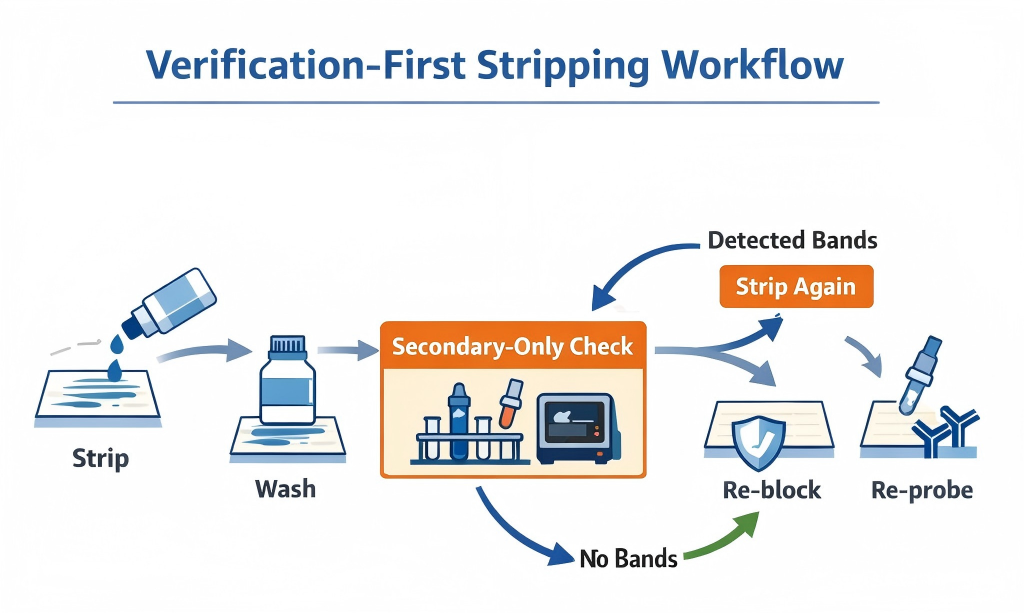
Verification-first workflow. Strip gently, wash thoroughly, then use a secondary-only check before re-probing. (Click to open full-size.)

Strip: Use the mildest condition that works.

Start with the mildest stripping condition that can remove bound antibodies. If you’re unsure, avoid defaulting to long incubations. Over-stripping can reduce recoverable signal and can also make background harder to control in later rounds.

Wash: Prioritize complete buffer exchanges.

Wash thoroughly in TBST (or your standard wash buffer). What matters most is not just wash time; it’s whether you are doing full solution exchanges to remove stripping reagents and any released antibody material. If you’re standardizing your workflow for consistency, your choice of buffers, substrates, membranes, and related essentials often lives in one place—your Western blot reagents setup.

What we mean by “buffer exchange”: replace the wash buffer with fresh TBST each time under agitation, rather than extending a single wash in the same buffer.

Verify: The secondary-only check that prevents ghost bands.

After stripping and washing, incubate the membrane with secondary antibody only (no primary), wash, then do a short exposure. This is the fastest, most reliable way to detect residual antibody signal before you invest in another full primary incubation.

Secondary-only check (operational definition): re-block the membrane, incubate with the same secondary used in round one (same species and detection chemistry), wash under the same rules, then take a short exposure that would have detected the original band. Use your round-one exposure as a reference point; the goal is to detect residual signal without overexposing the membrane. This check is only interpretable when the secondary and detection settings match what you used previously.

Table 3. Secondary-only check: how to confirm stripping worked

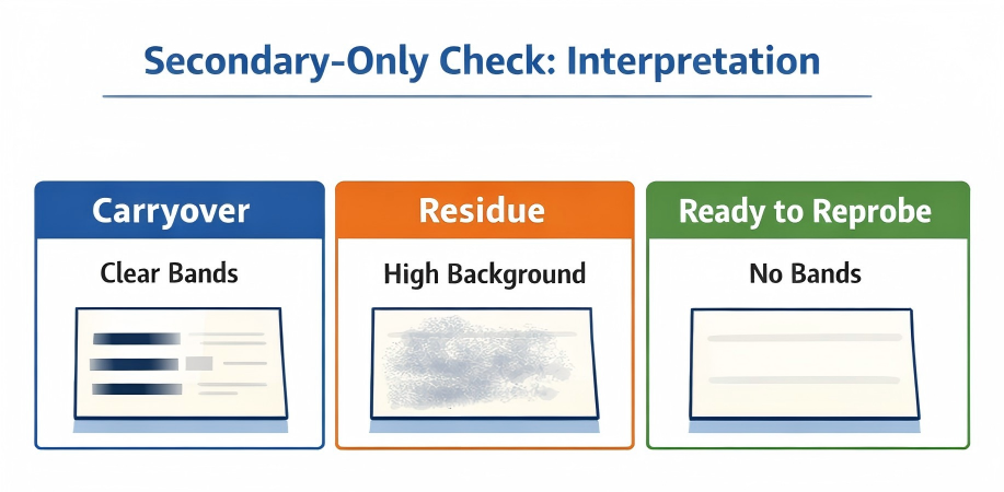
Secondary-only check. Use the pattern to decide whether to wash more, strip again, or proceed to re-probing. (Click to open full-size.)

Re-block and re-probe: Keep conditions conservative.

Re-blocking helps stabilize membrane surface behavior after stripping. When you re-probe, start with a validated antibody dilution rather than increasing concentration to “force” signal—on post-strip membranes, aggressive antibody concentrations often increase background faster than true signal.

Reprobing order tip: probe the most sensitive/low-abundance target first (before the membrane sees repeated processing), then reprobe higher-abundance targets or loading controls later. If phospho/total is your goal, phospho is typically probed first, then strip and probe total protein.

If your second round is aimed at a loading control, plan that choice deliberately. Many workflows rely on a stable loading control as the anchor for interpretation; for options that match your species and sample type, see Loading control antibodies. If your experiment depends on rigorous normalization across conditions, it also helps to align your strategy with Total protein normalization vs loading control antibodies before you decide which readout belongs in which round.

A realistic operating range is one to two reprobing rounds. Additional rounds can work, but signal loss and background drift become increasingly likely, especially for low-abundance targets.

Troubleshooting high background after stripping (and how to avoid ghost bands)

When reprobing fails, the symptom usually points directly to the correct lever. Ghost bands indicate antibody carryover, which is best addressed by washing and verification before escalating stripping strength. Weak second-round signal points toward over-stripping and calls for milder conditions or shorter exposure. Background haze commonly reflects residue and membrane surface effects, so washing and re-blocking dominate the fix. For pattern matching and upstream checks, the Western blot troubleshooting library is often the fastest way to identify whether you’re seeing carryover, non-specific binding, or a transfer/sample issue that stripping won’t solve.

If your experiment requires multiple targets with defensible comparability, the “one membrane, many rounds” strategy often stops being efficient. In those cases, rerunning separate blots—or outsourcing a critical target to a Western blotting service workflow—can be faster than repeated stripping iterations, especially when sample is limited or the target is low-abundance.

FAQ: western blot stripping buffer protocol and reprobing

What is a western blot stripping buffer, and what does it remove?

A western blot stripping buffer removes bound antibodies (primary and/or secondary) from the membrane so the blot can be probed again for a different target.

What is the best western blot stripping protocol for reprobing?

A reliable protocol uses the mildest stripping condition that works, thorough TBST washes with full exchanges, and a secondary-only verification step before reprobing.

How do you strip and reprobe a western blot without ghost bands?

Use a secondary-only check after stripping. If bands remain, improve washing first and repeat stripping incrementally before reprobing.

Why do I get high background after stripping a western blot?

High background is often caused by incomplete removal of stripping reagents, insufficient re-blocking, or overly concentrated antibod...

What is a Dilution Ratio?

Dilution ratio describes a simple dilution – a unit volume of solute (or sample) is combined with a desired unit volume of solvent (or diluent), to reach a desired total volume (Vsolute + Vsolvent = Total Vsolution)

Thus, a dilution ratio of 1:4 describes 1 part solute + 4 parts solvent = 5 parts total. The sum of both solute plus solvent equals total, f...

High background in DAB staining usually shows up as one of three patterns: a global brown/gray haze, edge-darkening, or granular brown speckling. The fastest way to fix it is to stop guessing and first identify which layer is generating the background: tissue chemistry, primary binding, the HRP detection/amplification layer, or...

Multiplex immunofluorescence (multiplex IF) rarely fails because you “missed a step.” It fails because you can’t reliably separate bleed-through, background, and true signal—and you don’t have a fast way to prove what’s actually happening.

Most multiplex problems are solved faster when you diagnose first: run the minimum controls, apply a few quick checks, then change the right lever in the right order. If you’re new to IF terminology, start here: immunofluorescence glossary. If you need a step-by-step workflow reference, use this resource (this post won’t repeat it): IHC/ICC/IF protocol resource.

• If you’re still selecting channels/fluors: multiplex fluorophore guide
• If you suspect autofluorescence: quick fixes guide

Quick answer: how to troubleshoot multiplex IF

What “failure” looks like in multiplex IF

Most multiplex issues fall into one (or more) of these patterns:

• Apparent co-localization everywhere (looks “too perfect”)
• One channel looks dirty (haze/grain) while others look fine
• Signal appears in the wrong compartment (e.g., nuclear-looking signal for a membrane marker)
• Weak target disappears when you adjust exposure to keep the bright target unsaturated
• Results change between runs even with the “same protocol”

When you see these, don’t change everything. Start by proving what kind of problem it is.

The minimum controls (must-have for multiplex)

You don’t need a dozen controls. You need the right ones.

1) Single-stain controls (non-negotiable)

What it is: Stain each target one at a time, using the same imaging settings you plan to use for multiplex.

What it tells you:

• Whether a channel is clean on its own
• Whether signal “leaks” into other channels (spillover/bleed-through)
• Whether your “co-localization” is real or optical/setting-driven

Use it like this (quick):

• Capture each single stain across all channels (not just the “expected” channel).
• If a single stain appears in another channel, that’s bleed-through (or detection cross-talk), not biology.

2) No-primary control (fast background reality check)

What it is: Run the full workflow without primary antibodies.

What it tells you:

• How much background comes from secondaries/detection, sample, or handling
• Whether your background problem is antibody-driven or system-driven

3) “Brightest-only” check (exposure trap detector)

What it is: Image only the brightest marker (or brightest single-stain) at the exposures you’re using for multiplex.

What it tells you:

• Whether imaging settings are forcing false positives in other channels
• Whether your bright marker is dominating the panel

Optional: Isotype control—useful when you suspect non-specific binding and your no-primary control is clean but staining still looks wrong. Don’t default to it as a first-line control.

Quick Checks: 5 minutes to identify the failure mode

Rule of thumb: Fix imaging QC (saturation + per-channel exposure rules) before changing staining variables.

Fix order that prevents endless reruns

When multiplex looks wrong, apply fixes in this order (least effort → biggest impact):

1. Imaging settings (QC first)
   • Remove saturation
   • Confirm no channel is “overdriving” the panel
2. Signal balance (make channels comparable)
   • Reduce the brightest target’s signal or imaging intensity before boosting the weakest
3. Specificity checks (controls-driven)
   • Single-stain + no-primary decide whether it’s bleed-through vs background
4. Only then adjust staining variables (dilution/incubation/washes)
   • One variable at a time, documented

Further reading (no overlap with this post): How to Choose Fluorophores for Multiplex IF. If what you’re seeing looks like tissue autofluorescence (broad, structure-like background), use this guide: 5 Tips to Reduce Autofluorescence.

Troubleshooting table: symptom → most likely cause → quickest fix

Multiplex immunofluorescence, or multiplex IF, often looks “simple” on paper—until channels start bleeding into each other, weak targets disappear, or background forces you to crank exposure. In reality, most multiplex failures come from three upstream issues: channel planning, where brightness is mismatched to abundance, overlap, including spectral spillover and crosstalk, and missing controls, meaning no single-stain proof. The goal is not “more color,” but clean, interpretable signal with defensible imaging rules—so your colocalization reflects biology, not artifacts.

This post is a practical workflow for fluorophore selection in multiplex IF: plan channels by abundance, prevent bleed-through, and validate with controls. It’s written as a microscope-side SOP—decision rules plus checks—not a fundamentals-only overview. If you want to align upstream variables first, start here: sample preparation for IHC/ICC/IF and cell/tissue fixation.

• Fluorophore fundamentals: spectra, brightness, photostability
• Single-stain controls: why they matter
• Troubleshooting workflow when background or spillover won’t behave

Quick answer: how to choose fluorophores for multiplex IF

Multiplex IF is a workflow: not just fluorophore choice

To make the intent clear: this post is a multiplex IF workflow—channel planning, single-stain spillover checks, and within-channel imaging consistency for comparisons. For fundamentals—what a fluorophore is, spectra basics, and selection basics— see how to choose the right fluorophore...

Western blot “quantification” is often treated like a software task. In reality, most wrong numbers come from two upstream issues: saturation (signal no longer scales with protein amount) and normalization (a reference that shifts or saturates). The goal is not “the darkest band,” but measurable signal in the linear range with a defensible reference—so your fold change reflects biology, not imaging artifacts.

This post is a practical, 5-minute workflow for western blot quantification: capture a quantifiable image, measure band intensity (densitometry), normalize (loading control or total protein), and calculate fold change. If you want broader context or need to fix blot quality first, these internal hubs are designed to be your next clicks:

• Western blotting technical resource center
• Western blot troubleshooting library
• Total protein normalization vs loading control antibodies (TPS vs LC)

...

Western blot “failures” are often blamed on antibodies, transfer, or blocking. But in many cases, the real bottleneck happens earlier: lysis choice plus lysate handling. A buffer that’s too mild can leave your target behind. A buffer that’s too harsh can produce viscous, debris-rich lysate that smears lanes and raises background. The goal is not “the strongest lysis possible,” but the mildest system that reliably extracts your target with the best signal-to-background—and then handling it in a way that keeps lanes clean.

This post is the very beginning for our Western blot experiment starting from sample prep. If you want broader context (or want to move downstream after lysate quality is solid), these internal hubs are designed to be your next clicks:

• Western blot sample preparation guide
...