This website uses cookies to ensure you get the best experience on our website.


- Table of Contents
Quantitative immunofluorescence | Imaging acquisition and data comparability
One IF sample looks faint at 100 ms, so you increase exposure to 300 ms. Another sample is bright enough at 100 ms. The resulting images look similar on screen—but can their fluorescence intensities be compared? Not from appearance alone. Exposure changes the amount of light recorded, and display adjustments can hide differences in the underlying measurements. To compare samples fairly, you need an acquisition range that works for both and a defensible relationship between their recorded pixel values. [1–3]
In camera-based fluorescence microscopy, exposure time determines how long the sensor collects light. Under stable illumination and within the detector's linear range, the light-dependent signal generally increases with exposure time. That includes fluorescence from the target, but also autofluorescence and optical background. A longer exposure may help with a faint signal when detector noise limits the measurement; it cannot distinguish target staining from nonspecific fluorescence. [1,3]
Exposure is not the only setting that affects the recorded image. Excitation intensity changes how much light reaches the specimen, while detector gain influences the recorded response in ways that depend on the instrument. Adjusting display contrast is different again: it can make an image look brighter without changing the underlying raw measurements. On a point-scanning confocal microscope, pixel dwell time, scan speed and averaging also govern signal collection. These distinctions matter when comparing images or trying to reproduce a setting on another instrument. [1,2]
If two specimens are imaged at different exposure times, their pixel values can differ even when their emitted fluorescence is similar. Detector offset, background and nonlinearity can further obscure the relationship. A brighter numerical reading therefore cannot be assigned to higher target abundance unless the acquisition conditions have been accounted for. [1,4]
Saturation is especially consequential. When a pixel reaches the recording ceiling, additional light no longer produces a higher stored value. Two structures with different true signals can therefore appear equally intense in the raw data. Reducing display brightness cannot retrieve the lost difference. Use the raw-image histogram or the microscope's range indicator, paying particular attention to the cells or regions that will actually be quantified. [1,3]
An image can also fail quantitatively at the opposite end of the range. If a faint signal is too close to autofluorescence, nonspecific staining or detector noise, small differences between samples may be unreliable even though no pixels are saturated. A useful exposure must accommodate both ends of the expected signal range: enough precision for dim specimens without clipping the brighter ones. [1,3]
Start with the experiment, not with the first attractive field of view. Examine representative specimens expected to give relatively bright and dim signals, and include the cellular regions you intend to measure. A strongly expressing positive control can help reveal saturation, but it is not necessarily a substitute for checking the brightest experimental condition. Samples should also be prepared and stained as consistently as the study design allows, since exposure cannot compensate for differences introduced before imaging. [1,3]
With objective, illumination, filters and detector mode set, begin at a short exposure and increase it while checking the raw-value distribution. Look for clipping in relevant regions, then inspect a dim specimen without changing the settings. Is its target-associated signal distinguishable from appropriate background, with sufficient precision for the intended comparison? If not, consider whether staining, illumination, detection or experimental design needs attention. A universal exposure time—or a fixed percentage of the detector's maximum—is not a sound substitute for this check. [1,3]
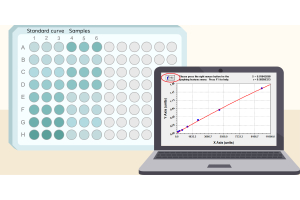
Next, assess whether the selected range supports quantitative measurement. A calibration or stable fluorescent reference may help establish how recorded intensity responds to exposure, but an apparently straight line from a few measurements is not enough if offset, background or bleaching has been overlooked. Repeated imaging of the same field can flag exposure-related signal loss; account for the additional light delivered during that test. The aim is to establish suitable conditions before acquiring the dataset, rather than attempting to repair avoidable problems afterward. [1,3]
Save the chosen settings and use them throughout the groups being compared. Locking exposure alone is insufficient if illumination, gain, optical configuration or acquisition processing changes. If one setting cannot capture both bright and dim structures acceptably, revisit the imaging strategy rather than letting automatic exposure choose a different value for each sample. Auto-exposure may improve how individual pictures look, but it undermines a straightforward comparison of their raw intensities. [1–3]
Matched acquisition settings make relative intensity comparisons more straightforward, provided relevant pixels are unsaturated and the signal can be measured adequately against background. Even then, differences in staining, sample handling, optical section thickness or region selection can affect the result. Fluorescence intensity is a measurement made under particular conditions; it is not automatically a direct measure of protein abundance. [1,3,4]
| Acquisition situation | Can the intensities be compared? | Practical decision |
|---|---|---|
| Same validated settings; no relevant saturation | Generally more suitable for relative comparison if relevant signals are measurable; sample preparation and analysis must also be comparable. | Use consistent background handling and analysis. |
| Different exposures; linear response and other conditions verified | Not as raw values alone. Comparison may be possible with validated calibration and correction. | Use a validated response model and appropriate corrections. |
| Different exposures; calibration or key metadata missing | Numerical comparability cannot be established from image appearance. | Prefer reacquisition with matched settings. |
| Important measurement regions saturated | Information lost through clipping cannot be recovered by exposure-time normalization. | Reimage at a suitable setting if quantitative comparison is needed. |
Take two groups photographed at 100 ms and 300 ms. A higher mean gray value in the 300 ms images does not establish higher target expression. A calibrated comparison may be possible if the instrument responds linearly over the relevant range, illumination and other settings are stable, and detector offset and background are handled appropriately. Simply dividing raw intensity by exposure time skips those checks. Nor can any calculation restore values that were clipped during acquisition. [1,4]
The question, then, is not whether the pictures look alike. It is whether the recorded signals can be placed on the same measurement scale, with assumptions that can be tested and reported.
The same software settings on two different days do not necessarily produce the same optical measurement. Light-source output can drift, alignment can change and detector readout modes may differ. Keep native image files and acquisition metadata, and record the objective, illumination and detection path, exposure or scanning settings, detector configuration and any processing applied during acquisition. These details make the measurements easier to interpret, repeat and audit. [2]
A stable fluorescent reference, imaged consistently, can help detect changes in instrument response between sessions. It does not compensate for shifts in antibody staining, sample preparation or target accessibility. Similarly, interleaving the order in which experimental groups are imaged can reduce the risk that gradual drift affects one group more than another. Neither measure makes separate staining batches inherently equivalent. [1–3]
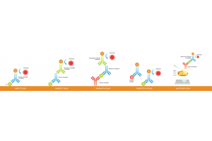
For multichannel experiments, select an appropriate acquisition setting for each fluorophore and keep that channel's protocol consistent across the specimens being compared. In indirect IF, fluorophore-conjugated secondary antibodies contribute to the spectral properties of each detection channel. Equal pixel values in different color channels do not imply equal fluorophore abundance or target expression. [1,2]
Before correcting a dataset, ask whether the information needed for the comparison was captured at all. If important regions are saturated, their higher intensities are lost. If weak signals are indistinguishable from background, the images may not support the intended comparison. And if settings changed without adequate calibration or metadata, a numerical correction may be impossible to justify. In these cases, reacquisition under a common protocol is generally preferable when feasible. [1,3,4]
There is a different case when native images are intact and the detector response has been calibrated over the relevant range. Here, a documented correction may be defensible. Preserve the raw files, state the model and assumptions, and report the processing. If images cannot be reacquired and a quantitative comparison remains uncertain, they may still be useful descriptively—but should not be presented as proof of a difference in protein expression. [2–4]
Good exposure settings do not make every image equally bright; they make meaningful intensity differences measurable. Check bright specimens for clipping and dim specimens for adequate signal before fixing the acquisition protocol. When exposures differ, use a validated measurement relationship rather than an appearance-based comparison. If that relationship cannot be established, acknowledge the limit or collect new images.
1. Jonkman J, Brown CM, Wright GD, Anderson KI, North AJ. Tutorial: guidance for quantitative confocal microscopy. Nature Protocols. 2020;15:1585–1611. https://doi.org/10.1038/s41596-020-0313-9
2. Montero Llopis P, Senft RA, Ross-Elliott TJ, et al. Best practices and tools for reporting reproducible fluorescence microscopy methods. Nature Methods. 2021;18:1463–1476. https://doi.org/10.1038/s41592-021-01156-w
3. Senft RA, Diaz-Rohrer B, Colarusso P, et al. A biologist’s guide to planning and performing quantitative bioimaging experiments. PLOS Biology. 2023;21:e3002167. https://doi.org/10.1371/journal.pbio.3002167
4. Culley S, Cuber Caballero A, Burden JJ, Uhlmann V. Made to measure: An introduction to quantifying microscopy data in the life sciences. Journal of Microscopy. 2024;295:61–82. https://doi.org/10.1111/jmi.13208