This website uses cookies to ensure you get the best experience on our website.


- Table of Contents
Your ELISA standard curve passes its checks. The diluted wells also fall within the assay’s quantitative range. Yet the same serum sample gives one concentration after a 1:2 dilution and a markedly different one after a 1:8 dilution. Which result should you use?
That discrepancy is the reason to examine dilutional parallelism. A well-fitting calibration curve describes the standards, not necessarily how an endogenous analyte behaves in a biological matrix. Testing a sample across dilutions can show whether the assay produces a concentration estimate that remains consistent enough for its intended use. It cannot, on its own, prove the estimate is accurate or identify the cause of a mismatch [1,2].
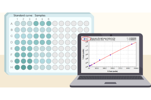
An ELISA calibration curve relates optical density to analyte concentration. Using it for serum, plasma or tissue extract assumes the endogenous target responds comparably to the reference material. That assumption may not hold: sample components can interfere with antibody binding or signal development, and endogenous proteins may differ from the calibrator in molecular form or binding state [1].
To examine parallelism, researchers dilute a sample containing endogenous analyte and compare its response with the assay’s calibration behavior. A practical first check is whether concentrations calculated for the original specimen agree across valid dilution points. Formal evaluations may instead, or additionally, compare dilution-response relationships with a predefined model and acceptance criteria. These approaches are related, but stable dilution-corrected values alone are not a complete curve-based parallelism assessment. Nor does parallelism require a four-parameter logistic (4PL) OD curve to be a straight line [1,3].
The distinction from other dilution experiments matters. Dilutional linearity is often tested using material containing added reference analyte, while spike recovery evaluates how much of an added quantity is measured. Parallelism generally concerns the behavior of endogenous analyte in its sample matrix. Definitions and experimental designs vary across immunoassay applications, so the report should state what was tested rather than rely on a label. None of these tests alone establishes antibody specificity [1,2].
Start with individual specimens containing enough endogenous analyte to yield several readings within the validated quantitative range. Include samples representative of the intended matrix and study population when material permits; a successful test on one unusually concentrated specimen says little about others. Respect any established minimum required dilution, then choose subsequent points that can still be measured reliably rather than clustering at the assay limits [1–3].
Twofold serial dilution is convenient, but there is nothing inherently definitive about that spacing. Choose it according to analyte abundance, assay range and available sample. Prepare dilutions consistently and measure replicates where feasible. For a more rigorous assessment, repeating independently prepared dilutions or testing across runs can help separate a persistent sample effect from an occasional pipetting or assay error [2,3].
Keep the underlying data: optical density, interpolated concentration in each diluted well, dilution factor and calculated concentration in the original specimen. Exclude values outside the assay’s established quantifiable range from the comparison. Multiplying an out-of-range estimate by its dilution factor does not make it valid.
For each valid dilution, multiply the interpolated well concentration by the total dilution factor. Table 1 uses hypothetical values to show this simple check. All measured values are assumed to fall within the assay’s usable quantitative range; the table illustrates agreement among corrected concentrations, not proof of formal curve parallelism.
| Dilution | Measured in well | Corrected original concentration |
|---|---|---|
| 1:2 | 120 pg/mL | 240 pg/mL |
| 1:4 | 62 pg/mL | 248 pg/mL |
| 1:8 | 31 pg/mL | 248 pg/mL |
Table 1. Hypothetical dilution series with relatively stable back-calculated concentration estimates.
In Table 1, the concentration measured in the well falls as expected, while the estimates for the original sample stay close: 240, 248 and 248 pg/mL. Now imagine another sample yielding corrected estimates of 190, 224, 269 and 310 pg/mL as dilution increases. That rising pattern needs investigation. It might reflect dilution-dependent matrix interference, a difference between endogenous analyte and calibrator, measurements near assay limits, or dilution errors. The trend alone cannot tell us which.

Figure 1. Simulated, dilution-corrected concentration profiles. Consistent estimates provide a useful screening observation; dilution-dependent drift warrants investigation. Neither profile is an experimental result or, by itself, a formal curve-based parallelism evaluation [1–3].
Researchers may summarize corrected concentrations using variation or relative deviation from a reference defined beforehand. In other settings, an analysis of the dilution-response curves is more appropriate. What counts as acceptable should follow the assay’s precision, reportable range and intended use—not a percentage cutoff borrowed without justification from a different validation setting. Requirements developed for regulated bioanalysis or vaccine assays may be informative without being universal rules for exploratory ELISA work [1–4].
One common explanation is matrix interference. As serum or plasma is diluted, the concentration of an interfering component also decreases, potentially changing how readily the assay detects the target. Corrected concentrations may therefore move toward a plateau at higher dilutions. Such a pattern is consistent with reduced interference, but it does not prove that the plateau represents the true concentration [1].
The endogenous protein itself may also differ from the calibrator. Isoforms, post-translational modifications, binding partners or protein complexes can affect access to the epitopes recognized by an antibody pair. Dilution might not remove those differences, and two apparently similar specimens may respond differently. A nonparallel result is therefore not, by itself, evidence of a defective reagent [1,3].
Before attributing the pattern to biology, check the measurement. Highly concentrated samples may exceed the validated response range; some sandwich assays can also exhibit a high-dose hook effect under relevant conditions. At the other end, uncertainty near the lower quantification limit becomes magnified when values are corrected for dilution. Poor mixing, transfer errors and between-run variability can produce apparent nonparallelism too [2].
A failure of agreement does not necessarily invalidate every dilution point. Suppose several adjacent, in-range dilutions give similar corrected estimates while less diluted wells do not. That may identify a candidate dilution interval for further evaluation—not a license to pick whichever value is preferred. Confirm its behavior using independent preparations, representative specimens and criteria appropriate to the intended use [1,3].
If estimates remain inconsistent across the usable range, averaging them only conceals the disagreement. Investigate before reporting a concentration, or qualify the result if the study allows. Additional dilution might reduce interference but also push the target below the lower quantification limit, leaving no usable dilution. An alternative assay or an independent measurement may then be necessary.
Even close agreement across dilutions establishes only part of the case. It does not demonstrate absolute accuracy, molecular specificity or equivalence between sample analyte and calibrator. Precision, selectivity and recovery evidence may still be needed, depending on the purpose of the measurement [1,2].
First ask whether the pattern repeats. Prepare the dilution series again, check which points are truly quantifiable and examine individual specimens rather than only a pooled sample. If disagreement affects only some specimens, investigate their matrices or endogenous analyte forms. If it occurs across the intended population, calibration and assay design warrant closer examination [1,3].
Changes to dilution factor or diluent sometimes lessen interference, but can also reduce the measurable target or alter the matrix in a new way. Recheck the relevant performance characteristics after a meaningful change, including precision, quantification limits and dilution behavior. If sample and calibrator responses remain incompatible, revisiting the reference material, antibody pair or assay format may be more productive than further dilution trials [1,3].
The point is not to make the numbers agree at any cost. It is to learn where the method supports a concentration estimate—and where it does not.
A clean standard curve is necessary, but it cannot establish how every real sample behaves. Dilutional parallelism adds evidence about whether endogenous analyte can be quantified consistently against the assay’s reference material. Considered alongside precision, quantification limits and other fit-for-purpose validation data, it helps distinguish a defensible sample concentration from one that still needs investigation.
[1] Tu J, Bennett P. Parallelism experiments to evaluate matrix effects, selectivity and sensitivity in ligand-binding assay method development: pros and cons. Bioanalysis. 2017;9(14):1107–1122. doi:10.4155/bio-2017-0084.
[2] Andreasson U, Perret-Liaudet A, van Waalwijk van Doorn LJC, et al. A practical guide to immunoassay method validation. Front Neurol. 2015;6:179. doi:10.3389/fneur.2015.00179.
[3] Stevenson LF, Purushothama S. Parallelism: considerations for the development, validation and implementation of PK and biomarker ligand-binding assays. Bioanalysis. 2014;6(2):185–198. doi:10.4155/bio.13.292.
[4] Dessy F, Sonderegger I, Wagner L, et al. Harmonization of vaccine ligand binding assays validation. Bioanalysis. 2024;16(19–20):1067–1091. doi:10.1080/17576180.2024.2411925. (Vaccine immunogenicity assay context.)