This website uses cookies to ensure you get the best experience on our website.


- Table of Contents
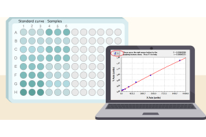
Your ELISA standard curve looks convincing, yet two wells containing the same sample give noticeably different readings. Is the sample unreliable, or is something wrong with the plate? Start with the raw OD values, where the sample falls on the calibration curve, and whether other samples show the same problem. Those checks are more useful than immediately changing the protocol.
A smooth standard curve is reassuring, but it is not a test of precision for each unknown sample. Standards establish the calibration relationship; controls and sample replicates provide additional evidence about assay performance. Even when the fitted curve looks good, an individual sample pair may remain unreliable [1,2].
The coefficient of variation (CV) expresses standard deviation relative to the mean: CV (%) = 100 × SD / mean. With only two wells, it summarizes the difference between those two readings. It cannot reliably characterize the precision of an entire assay, which must be assessed across repeated measurements under defined conditions [2].
Before interpreting the percentage, look at the actual OD readings. When the mean signal is near zero, a small absolute difference can produce a large CV. Background subtraction can make this especially apparent if the remaining net signal is very small. In that situation, the more important question is whether the sample is within the validated quantification range at all [2].
For example, two hypothetical OD pairs—0.10 and 0.14, versus 1.00 and 1.04—have the same absolute difference of 0.04. Using the sample standard deviation (n = 2), their CVs are approximately 23.6% and 2.8%, respectively. These values illustrate the arithmetic only; they are not experimental results or acceptance limits. Background correction and conversion through a nonlinear calibration curve can change the interpretation further.
OD CV and concentration CV are not interchangeable. When a nonlinear ELISA calibration curve is relatively flat, a small OD difference may correspond to a much larger difference in interpolated concentration. Follow the method’s specified approach for replicate calculations and acceptance; keep both raw OD and calculated concentration available when investigating a discrepancy [1,2,4].
A single disagreeing pair does not identify its cause. An ELISA experimental design checklist can help document the plate map, which is often more informative: do affected samples cluster at low signal, follow a row or column, occur near a dispensing transition, or appear scattered without an obvious pattern?
| What you observe | What to investigate first | What it does not establish |
|---|---|---|
| One isolated sample pair differs | Sample mixing, aliquoting, individual well condition and sample matrix | That a specific pipetting step failed |
| Low-signal samples frequently show high CV | Raw net signal, background and established lower quantification limit | That the large CV necessarily reflects biological variability |
| Disagreement follows rows, columns or dispensing order | Plate position, wash performance, incubation and timing records | Which process created the pattern |
| Calibrators or QCs also disagree | Possible run-wide or shared procedure problem | That the entire run is invalid without applying its predefined QC rules |
| Curve fit looks good, but particular samples disagree | Sample-specific factors and individual well handling | That the curve fit validates the unknown samples |
Position matters. Lilyanna and colleagues observed location-dependent assay responses in the specific commercial plates and chemiluminescent sandwich ELISA they studied [5]. This illustrates why a possible ELISA edge effect or another positional pattern is worth examining, but it does not mean plate-surface variation is the cause of a particular absorbance ELISA result. Dispensing, washing and timing histories should be examined alongside the plate map.
An isolated mismatch may be a local event, while a recurring directional pattern raises suspicion of a shared procedural or positional influence. Neither pattern identifies the cause without a controlled check.
The two wells need equivalent sample aliquots and comparable treatment throughout the assay. If the sample was not well mixed, or if dispensing was inconsistent, the wells may start with different amounts of material. Viscous samples and very small dispensing volumes deserve particular attention. These are plausible sources of variation, not conclusions that can be drawn from a high CV alone [3].
Variation can also arise after sample addition. Unequal washing—one of the well-to-well variation factors covered in the PicoKine ELISA troubleshooting guide—may leave different amounts of residual liquid or unbound reagent, while a bubble in the optical path can affect a plate-reader measurement. Checking the wells and wash record is more useful than assuming the sample itself caused the disagreement.
ELISA pipetting order and timing can matter when paired wells are handled at different points in a dispensing sequence. What matters is whether each well experiences a comparable effective reaction interval—not simply whether reagents were added at exactly the same clock time. Check the addition and stop sequence when a directional trend appears.
When standards and controls are acceptable but certain specimens remain inconsistent, sample matrix interference—one of the issues addressed by appropriate ELISA controls—is another possibility. Standards prepared in assay buffer may not reproduce every biological sample. Evidence for matrix interference requires additional work, such as suitable dilution or recovery checks; a disagreeing pair does not establish it [2].
Begin with the raw data: confirm the well assignments, sample dilution, blank correction and original readings. Check whether either signal is outside the usable range or whether a bubble or other visible well problem was recorded. Do not discard one replicate merely because it differs from the other.
Next, look beyond that pair. If the run meets its calibration and QC rules while only one sample is inconsistent, a targeted repeat may answer the question without rerunning everything. If multiple samples share a plate-position or processing pattern, examine the relevant dispensing, washing and timing records. Failed QCs require the method’s run-level rules rather than an ad hoc decision [1,2].
Choose the next repeat to test a specific explanation. A fresh mixed aliquot can check sample handling; a dispensing performance check can address pipetting; a deliberately changed plate position can test for positional bias. Keep unrelated conditions fixed so the outcome can be interpreted.
Document the change and the result. If agreement improves, it supports further investigation of that factor; it does not prove the entire method is now precise. Repeatability and intermediate precision are broader properties that require a planned study [2].
A duplicate pair that fails its predefined acceptance criteria requires a documented response, not a choice of whichever well better matches expectations. Check the sample’s quantification range, the run QC results and the method’s repeat rules. A mean concentration within range does not override a prespecified replicate-agreement rule [1,2].
If there is documented evidence of a technical failure, follow the method’s established rules for invalidation or retesting. Without such evidence, excluding a high or low well simply because it is inconvenient can bias the result. If no valid sample result can be obtained, report the limitation rather than inventing a defensible-looking concentration.
Singlet testing is a separate design question. Pillutla and colleagues evaluated when a singlet approach may be appropriate for validated ligand-binding assays with sufficiently characterized precision [6]. This does not justify replacing a failed duplicate pair with one convenient well. Replicate strategy and acceptance criteria belong to the specific method and its intended use.
When ELISA duplicates disagree despite a good-looking standard curve, check the raw OD, quantification range and plate-wide pattern before touching the protocol. The right next step is a targeted check that distinguishes plausible causes—not automatic rejection of a well or an unnecessary repeat of the full plate.
[1] Azadeh M, Gorovits B, Kamerud J, et al. Calibration Curves in Quantitative Ligand Binding Assays: Recommendations and Best Practices for Preparation, Design, and Editing of Calibration Curves. The AAPS Journal. 2018;20:22. doi:10.1208/s12248-017-0159-4. https://doi.org/10.1208/s12248-017-0159-4
[2] Dessy F, Sonderegger I, Wagner L, et al. Harmonization of Vaccine Ligand Binding Assays Validation. Bioanalysis. 2024;16(19-20):1067–1091. doi:10.1080/17576180.2024.2411925. https://doi.org/10.1080/17576180.2024.2411925
[3] Aydin S, Emre E, Ugur K, et al. An overview of ELISA: a review and update on best laboratory practices for quantifying peptides and proteins in biological fluids. Journal of International Medical Research. 2025;53(2):3000605251315913. doi:10.1177/03000605251315913. https://doi.org/10.1177/03000605251315913
[4] Xiang Y, Donley J, Seletskaia E, et al. A Simple Approach to Determine a Curve Fitting Model with a Correct Weighting Function for Calibration Curves in Quantitative Ligand Binding Assays. The AAPS Journal. 2018;20:45. doi:10.1208/s12248-018-0208-7. https://doi.org/10.1208/s12248-018-0208-7
[5] Lilyanna S, Ng EMW, Moriguchi S, et al. Variability in Microplate Surface Properties and Its Impact on ELISA. The Journal of Applied Laboratory Medicine. 2018;2(5):687–699. doi:10.1373/jalm.2017.023952. https://doi.org/10.1373/jalm.2017.023952
[6] Pillutla R, Gorovits B, Gleason C, et al. Recommendations for Singlet-Based Approach in Ligand Binding Assays: An IQ Consortium Perspective. Bioanalysis. 2020;12(12):823–834. doi:10.4155/bio-2020-0094. https://doi.org/10.4155/bio-2020-0094